3 Using SIPmg R package
This R package was designed to facilitate statistical analyses using SIP metagenomic data. Particularly, coverage and taxonomic classification of metagenome-assembled genomes and metadata of fractionated DNA is used to identify incorporators and quantify isotopic enrichment.
Overall, the package can perform the following:
Coverage normalization to absolute concentrations or relative coverage. Scaling of coverages to absolute abundances based on post-fractionation reference standards, called sequins.
Statistical analysis based on either of
- AFE mathematical model by Hungate et al. (2015) or
- Delta buoyant density \(AFE_{ΔBD}\) = \(\frac{W_{Lab}- W_{Light}}{I_{max}}\).
Where Imax is the maximum linear shift in DNA BD (upon 100% labeling), as discussed by Birnie and Rickwood (1978) - Analyses as offered by HTS-SIP
- Data visualization for identification of isotope incorporators.
3.1 Example workflow
qSIP analysis is typically performed using sequins, MAG coverage, and MAG taxonomy is performed using this R markdown. Briefly, coverages are normalized, MAG coverages are then scaled based on linear regression models from sequin coverage and concentrations, a phyloseq object is created from MAG absolute concentrations and taxonomy (GTDB taxonomy output format is required) data.
Note: Sequins that were spiked in the DNA-SIP fractions will be used in scaling and creating linear regression models for evaluating absolute MAG concentrations. Please see sequin_scaling.R
For normalizing coverage values please see pooling_funs.R
This R markdown primarily uses Tidyverse, phyloseq, and HTSSIP packages
This markdown uses functions from functions_qSIP_MAGs.R
For this data, MetaSIPSim (developed by Barnett et al, 2020) was used to simulate a data set from a hypothetical SIP workflow performed on the MBARC-26 mock community (as defined in Singer et al, 2016). The data set was further augmented with simulated post-fractionation sequin spike-ins and the data set was simulated to have all 26 organisms as incorporators. Some of the 26 organisms also had plasmids, which were assembled as distinct genomic units, adding the total genomic features in the simulated study to be 38
#Load required libraries

list.of.packages <- c("tidyverse", "HTSSIP", "ggpubr","data.table")
new.packages <- list.of.packages[!(list.of.packages %in% installed.packages()[,"Package"])]
if(length(new.packages)) install.packages(new.packages, quiet = T, dependencies = T, repos = "http://cran.us.r-project.org")

if (!require("BiocManager", quietly = TRUE))
    install.packages("BiocManager")
BiocManager::install("phyloseq")

library(tidyverse)
library(phyloseq)
library(HTSSIP)
library(ggpubr)
library(SIPmg)


set.seed(seed = 1000)
3.2 Load required data
The following files are required:
3.2.1 MAG coverage data
Pooled coverages data as a comma separated file (.csv file) across samples for Features including sequins that were used as spike-ins. The followings columns are required:
Feature: A character string describing the
FeaturelabelSample: The label for these n number of columns should be in the format of “‘isotope’_rep_#_fraction_#”. For instance, “12C_rep_1_fraction_1”. The number of sample columns should be the same as the product of (replicates, fractions, isotopes)
3.2.2 Sequin metadata
Load the sequins metadata as a comma separated file (.csv file) which has the following columns:
Feature: As described above
Length: Length of the sequin in bp
GC_content: GC content of the sequin
Sequence: Sequin nucleotide sequence
Concentration: Concentration of the sequin in attamoles/uL
3.2.3 Dilutions data
Load dilutions data as a comma separated file (.csv file) that contains the following columns
Sample: Similar to the sample name as described above.
Dilution: Dilution of sequins added to the fraction before sequencing.
3.2.4 Fractions metadata
A fractions file as a comma separated file (.csv file) with the following columns:
Replicate: Depends on how many replicates the study has
Fractions: Typically in the range of 1-24
Buoyant_density: As calculated from the refractometer for each fraction and replicate
Isotope - “12C”, “13C”, “14N”, “15N” etc.
DNA_concentration
Sample - In the format “‘isotope’_rep_#_fraction_#”. For instance 12C_rep_1_fraction_1
3.2.5 GTDB style taxonomy data
A taxonomy file in the GTDB output format (.tsv format). Load the bacteria and archaea taxonomy outputs separately. The markdown requires loading the standard output files from GTDB-Tk separately for bacteria and archaea
3.2.6 MAG absolute concentrations
MAG absolute concentrations obtained from scaling_sequins.R.
mag_tab object obtained from the above script is to be used as the input here
3.2.7 GC content
GC content of the MAGs as a comma separated file (.csv file). The table should contain the following columns:
OTU: MAG identifier such as the
Featurelabel from thesequin_scaling.RscriptGC_content: GC content of the
Featurein the range of 0-1
3.2.8 Log scale BOOLEAN
True or False depending on how you would want the MAG coverages to be scaled. Select TRUE if you need MAG concentrations scaled on the log scale
3.2.9 Coefficient of variation
Acceptable coefficient of variation for coverage and detection (eg. 20 for 20 % threshold of coefficient of variation)
Coverages above the threshold value will be flagged in the plots. Here a value of 20 is used.
## Load data
#Coverage metadata
#Uncomment if your coverage data is in the format mentioned above for this file. Remains commented if you are using the output from `checkm coverage`
f_tibble <- readr::read_csv("mock_input_data/coverage_metadata.csv")

#Sequins metadata
sequins <- readr::read_csv(file="mock_input_data/sequins_metadata.csv")

#Dilutions data
seq_dil = readr::read_csv(file = "mock_input_data/dilutions_data.csv")

#Log scale BOOLEAN. True or False depending on how you would want the MAG coverages to be scaled. Select TRUE if you need MAG concentrations scaled on the log scale
log_scale = TRUE

#coe_of_variation. Acceptable coefficient of variation for coverage and detection (eg. 20 - for 20 % threshold of coefficient of variation) (Coverages above the threshold value will be flagged in the plots)
coe_of_variation = 20

#Taxonomy
gtdbtk_bac_summary = readr::read_delim("mock_input_data/gtdbtk.bac120.summary.tsv",
                                 "\t", escape_double = FALSE, trim_ws = TRUE)
gtdbtk_archaea = readr::read_delim("mock_input_data/gtdbtk.ar122.summary.tsv",
                             "\t", escape_double = FALSE, trim_ws = TRUE)
#GC content
GC_content <- readr::read_csv(file = "mock_input_data/GC_content.csv")

#Fractions
fractions = readr::read_csv("mock_input_data/fractions.csv")
3.3 Coverage normalization and scaling
Coverage data of MAGs (or features of interest) and sequins is scaled using sequin concentration to obtain absolute concentration of MAGs (or features of interest). For this step, either linear regression or robust linear regression can be used.
If linear regression is used, the function scale_features_lm is used. The functions in sequin_scaling_lm.R are used for this step.
If robust linear regression is used, the outliers impact on the regression models is minimized. For robust linear regression, scale_features_rlm is used. The functions in sequin_scaling_rlm.R are used for this step. In this example workflow, robust linear regression is used to scale coverage data in log10 scale.
For more discussion on the choice of regression method and comparison of the two methods please see this vignette
3.3.1 This function uses the following datasets:
- Coverage data (
f_tibble) - Sequins metadata (
sequins) - Dilution of sequins used to add into the fractions (
seq_dil)
The regression scaling plots are saved in the project folder within a subfolder sequin_scaling_plots
taxonomy_tibble = dplyr::bind_rows(gtdbtk_bac_summary, gtdbtk_archaea) #Combine bacteria and archaea taxonomy files if it has not been done yet
#mag_tab is a tibble with absolute concentrations of MAGs obtained by scaling MAG coverages using linear regression models on sequin coverages and concentration

##Scale MAG coverages to obtain MAG absolute concentrations and save scaling plots in the working directory
#For rlm scaling using scale_features_rlm
#For rlm scaling using scale_features_lm
mag_tab_scaled <- SIPmg::scale_features_rlm(f_tibble, sequins, seq_dil, log_scale, coe_of_variation = coe_of_variation, save_plots = FALSE)
mag_tab = as.matrix(mag_tab_scaled$mag_tab) #Extract absolute abundances as a matrix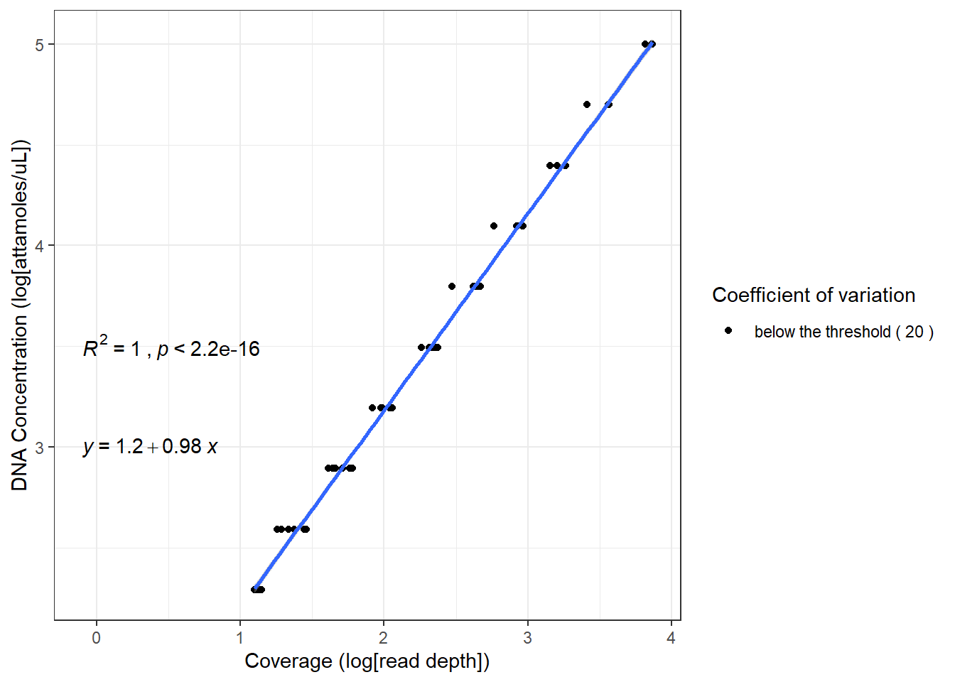
3.4 Preparation of scaled data for qSIP analysis
The scaled abundance data, taxonomy data, and metadata is then converted to phyloseq objects and a master phyloseq object is created for qSIP analysis.
mag.table = phyloseq::otu_table(mag_tab, taxa_are_rows = TRUE) #Phyloseq OTU table

taxonomy.object = SIPmg::tax.table(taxonomy_tibble) # Create a taxonomy phyloseq object
samples.object = SIPmg::sample.table(fractions) # Create a samples phyloseq object
phylo.qSIP = SIPmg::phylo.table(mag.table, taxonomy.object, samples.object) # Make a phyloseq table for downstream qSIP analysis
3.5 Estimation of atom fraction excess
The following steps estimate the atom fraction excess (AFE) in the MAGs. This calculation is based on the mathematical model suggested by Hungate et al. (2015). In the article, the authors suggest that GC contents of the individual biological features of interest should be accounted for to have a better estimate of AFE. Through the power of metagenomic analysis and the recovery of MAGs, one can estimate the GC content of features of interest and thereby obtain a better estimate of AFE. Thus, here the user would use the GC contents of MAGs in the AFE estimations and obtain isotopic enrichment of individual MAGs.
An important consideration is that the AFE calculations are based on a mathematical model and are not an absolute estimate of isotopic enrichment. One of the goals of AFE estimation is to determine isotope incorporators.
In this example workflow, the approach reported in Hungate et al. (2015) is used to determine incorporators.
For this step, the following are used:
- Master phyloseq object from the previous step
- GC content
Thanks to HTSSIP R package, bootstrapping can be performed faster with multithreading.
atomX = SIPmg::qSIP_atom_excess_MAGs(phylo.qSIP,
                               control_expr='Isotope=="12C"',
                               treatment_rep='Replicate',
                               Gi = GC_content)
#Bootstrap confidence intervals
df_atomX_boot = SIPmg::qSIP_bootstrap_fcr(atomX, n_boot=10) #Change "parallel = FALSE" to compute using a single-core
3.6 Plot the atom fraction excess plot
Plot the atom fraction excess data with 5 % and 95 % quantiles as the confidence limits. In the same way as reported in Hungate et al. (2015), a MAG is considered an incorporator if the lower confidence interval of its AFE is above zero.
CI_threshold = 0
df_atomX_boot = df_atomX_boot %>%
  dplyr::mutate(Incorporator = A_CI_fcr_low > CI_threshold,
         OTU = reorder(OTU, -A))

(atom_f_excess_plot = ggplot2::ggplot(df_atomX_boot, aes(OTU, A, ymin=A_CI_low, ymax=A_CI_high, color=Incorporator)) +
  geom_pointrange(size=0.25) +
  geom_linerange() +
  geom_hline(yintercept=0, linetype='dashed', alpha=0.5) +
  labs(x='MAGs', y='Atom fraction excess') +
  theme_bw() +
  coord_flip() +
  ggtitle("Isotope incorporating MAGs"))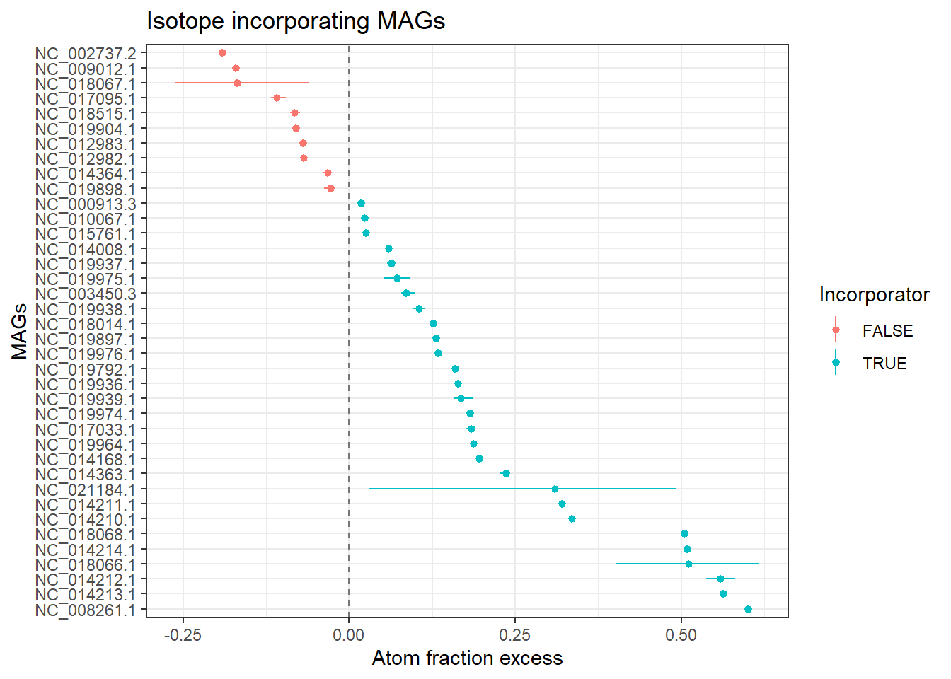
3.7 Check incorporator list
#Get incorporator info
n_incorp = df_atomX_boot %>%
  dplyr::filter(Incorporator == TRUE) %>%
  nrow
#Get incorporator list
incorporator_list = SIPmg::incorporators_taxonomy(taxonomy = taxonomy_tibble, bootstrapped_AFE_table = df_atomX_boot)
#Print incorporator information
cat('Number of incorporators:', n_incorp, '\n')
## Number of incorporators: 28print(incorporator_list, n = nrow(incorporator_list))## # A tibble: 28 × 2
## OTU taxonomy
## <fct> <chr>
## 1 NC_000913.3 Terriglobusroseus
## 2 NC_003450.3 Segniliparusrotundus
## 3 NC_008261.1 Nocardiopsisdassonvillei
## 4 NC_010067.1 Olsenellauli
## 5 NC_014008.1 Meiothermus_Bsilvanus
## 6 NC_014168.1 Meiothermus_Bsilvanus
## 7 NC_014210.1 Hungateiclostridiumthermocellum
## 8 NC_014211.1 Clostridium_Pperfringens
## 9 NC_014212.1 Desulfosporosinusacidiphilus
## 10 NC_014213.1 Desulfosporosinusacidiphilus
## 11 NC_014214.1 Desulfosporosinusacidiphilus
## 12 NC_014363.1 Desulfosporosinusmeridiei
## 13 NC_015761.1 Streptococcuspyogenes
## 14 NC_017033.1 Thermobacilluscomposti
## 15 NC_018014.1 Hirschiabaltica
## 16 NC_018066.1 Hirschiabaltica
## 17 NC_018068.1 Salmonellaarizonae
## 18 NC_019792.1 Pseudomonas_Astutzeri_AE
## 19 NC_019897.1 Pseudomonas_Astutzeri_AE
## 20 NC_019936.1 Frateuriaaurantia
## 21 NC_019937.1 Sediminispirochaetasmaragdinae
## 22 NC_019938.1 Fervidobacteriumpennivorans
## 23 NC_019939.1 Coraliomargaritaakajimensis
## 24 NC_019964.1 Halovivaxruber
## 25 NC_019974.1 Natronobacteriumgregoryi
## 26 NC_019975.1 Natronococcusoccultus
## 27 NC_019976.1 Natronococcusoccultus
## 28 NC_021184.1 NatronococcusoccultusIt appears that not all incorporators were identified with the bootstrapping method. This could be due to the model unable to detect the incorporators. Another way to detect incorporators, as mentioned above, is to test with the ΔBD method or with the HR-SIP or MW-HR-SIP methods. For a more detailed discussion, please refer this vignette
sessionInfo()## R version 4.2.2 (2022-10-31 ucrt)
## Platform: x86_64-w64-mingw32/x64 (64-bit)
## Running under: Windows 10 x64 (build 19044)
##
## Matrix products: default
##
## locale:
## [1] LC_COLLATE=English_Canada.utf8 LC_CTYPE=English_Canada.utf8
## [3] LC_MONETARY=English_Canada.utf8 LC_NUMERIC=C
## [5] LC_TIME=English_Canada.utf8
##
## attached base packages:
## [1] stats graphics grDevices utils datasets methods base
##
## other attached packages:
## [1] SIPmg_1.4 ggpubr_0.5.0 HTSSIP_1.4.1
## [4] phyloseq_1.42.0 forcats_0.5.2 stringr_1.5.0
## [7] dplyr_1.0.10 purrr_0.3.5 readr_2.1.3
## [10] tidyr_1.2.1 tibble_3.1.8 ggplot2_3.4.0
## [13] tidyverse_1.3.2 BiocManager_1.30.19
##
## loaded via a namespace (and not attached):
## [1] readxl_1.4.1 backports_1.4.1
## [3] plyr_1.8.8 igraph_1.3.5
## [5] lazyeval_0.2.2 splines_4.2.2
## [7] BiocParallel_1.32.4 GenomeInfoDb_1.34.4
## [9] digest_0.6.30 foreach_1.5.2
## [11] htmltools_0.5.4 fansi_1.0.3
## [13] magrittr_2.0.3 memoise_2.0.1
## [15] googlesheets4_1.0.1 cluster_2.1.4
## [17] tzdb_0.3.0 Biostrings_2.66.0
## [19] annotate_1.76.0 modelr_0.1.10
## [21] matrixStats_0.63.0 vroom_1.6.0
## [23] timechange_0.1.1 colorspace_2.0-3
## [25] blob_1.2.3 rvest_1.0.3
## [27] haven_2.5.1 xfun_0.35
## [29] crayon_1.5.2 RCurl_1.98-1.9
## [31] jsonlite_1.8.4 survival_3.4-0
## [33] iterators_1.0.14 ape_5.6-2
## [35] glue_1.6.2 gtable_0.3.1
## [37] gargle_1.2.1 zlibbioc_1.44.0
## [39] XVector_0.38.0 DelayedArray_0.24.0
## [41] car_3.1-1 Rhdf5lib_1.20.0
## [43] BiocGenerics_0.44.0 abind_1.4-5
## [45] scales_1.2.1 DBI_1.1.3
## [47] rstatix_0.7.1 Rcpp_1.0.9
## [49] xtable_1.8-4 bit_4.0.5
## [51] stats4_4.2.2 httr_1.4.4
## [53] RColorBrewer_1.1-3 ellipsis_0.3.2
## [55] farver_2.1.1 pkgconfig_2.0.3
## [57] XML_3.99-0.13 sass_0.4.4
## [59] dbplyr_2.2.1 locfit_1.5-9.6
## [61] utf8_1.2.2 labeling_0.4.2
## [63] polynom_1.4-1 tidyselect_1.2.0
## [65] rlang_1.0.6 reshape2_1.4.4
## [67] AnnotationDbi_1.60.0 munsell_0.5.0
## [69] cellranger_1.1.0 tools_4.2.2
## [71] cachem_1.0.6 cli_3.4.1
## [73] generics_0.1.3 RSQLite_2.2.19
## [75] ade4_1.7-20 broom_1.0.1
## [77] evaluate_0.19 biomformat_1.26.0
## [79] fastmap_1.1.0 yaml_2.3.6
## [81] knitr_1.41 bit64_4.0.5
## [83] fs_1.5.2 KEGGREST_1.38.0
## [85] nlme_3.1-160 xml2_1.3.3
## [87] compiler_4.2.2 rstudioapi_0.14
## [89] png_0.1-8 ggsignif_0.6.4
## [91] reprex_2.0.2 geneplotter_1.76.0
## [93] bslib_0.4.2 stringi_1.7.8
## [95] highr_0.10 lattice_0.20-45
## [97] Matrix_1.5-3 vegan_2.6-4
## [99] permute_0.9-7 multtest_2.54.0
## [101] vctrs_0.5.1 pillar_1.8.1
## [103] lifecycle_1.0.3 rhdf5filters_1.10.0
## [105] jquerylib_0.1.4 data.table_1.14.6
## [107] bitops_1.0-7 GenomicRanges_1.50.1
## [109] R6_2.5.1 bookdown_0.31
## [111] IRanges_2.32.0 codetools_0.2-18
## [113] MASS_7.3-58.1 assertthat_0.2.1
## [115] rhdf5_2.42.0 SummarizedExperiment_1.28.0
## [117] DESeq2_1.38.1 withr_2.5.0
## [119] S4Vectors_0.36.1 GenomeInfoDbData_1.2.9
## [121] mgcv_1.8-41 parallel_4.2.2
## [123] hms_1.1.2 grid_4.2.2
## [125] rmarkdown_2.19 MatrixGenerics_1.10.0
## [127] carData_3.0-5 googledrive_2.0.0
## [129] Biobase_2.58.0 lubridate_1.9.0